For years, the biggest players in CPG (Consumer Packaged Goods) and FMCG: Unilever, Nestlé, Kraft Heinz built their empires on food. But now? They’re making a massive pivot..if you had told me 5 years ago that these brands would be pulling back from food, I would’ve raised an eyebrow.
-Unilever is cutting loose its $8 billion ice cream division, choosing to focus on higher-margin beauty and wellness.
-Nestlé is doubling down on health-science-based nutrition as food brands struggle with pricing power.
- CPG giants are seeing stronger growth in self-care, supplements, and skincare than in traditional food categories.
The global personal care market is expected to hit $758 billion by 2030, while processed food growth slows.
Why This Shift?
1. Margins in food are shrinking. Consumers are trading down, private labels are winning, and inflation-wary shoppers aren’t absorbing cost hikes like they used to.
2. Health & wellness are driving premiumization. Customers will pay more for skincare, supplements, and functional beverages—but not for basic pantry staples.
3. Brand loyalty in food is eroding. Over 50% of consumers are comfortable switching food brands based on price, but loyalty remains strong in beauty, healthcare, and wellness.
Winning Brands Are Already Moving:
-L'Oréal’s skincare division posted 9.1% revenue growth last year, while traditional CPG food brands saw single-digit declines.
-The Coca-Cola Company is investing in functional drinks and non-carbonated wellness categories to stay relevant.
-PepsiCo’s biggest success? Gatorade’s expansion into hydration and performance-based drinks, not soda.
CPG Leaders:
✅ Stop thinking of food as the core driver of growth. Instead, align with evolving consumer behavior. ✅ Invest in personalization, self-care, and functional health. That’s where demand (and pricing power) is strongest. ✅ Rethink your brand mix. Is your portfolio weighted toward categories that will still be relevant in 5-10 years?
So, here’s my question to FMCG execs: Are you future-proofing your brand strategy or just managing decline?
https://tinyurl.com/5d8s5ytn
Something's happening in CPG. The legacy giants are dramatically under-pacing the market, while a new generation of startups is sprinting ahead.
This isn't just a quarterly anomaly. It's a fundamental shakeup. The old playbook—brute-force distribution and massive ad budgets—is broken. The power has shifted from the brand to the consumer.
In our latest newsletter, we dive into the why:
1. Consumers are now Curators: They demand transparency and trust. 2. Agility is the new Scale: Startups can innovate in weeks, not years. 3. Connection is the new Currency: Community is beating traditional advertising.
This CPG shakeup is a lesson for every industry, from food & bev to healthcare. The old guard is learning that their greatest strength (massive size) has become their greatest liability.
A natural monopoly occurs when a single firm can produce and distribute a specific product or service more efficiently and economically than multiple competing firms. In such markets, the cost structure and economies of scale are such that average total costs decrease as the firm’s output increases. This means that as the natural monopoly produces more, the cost per unit of production decreases.
The term “natural” in natural monopoly refers to the inherent characteristics of the industry or service that make it naturally conducive to a single, dominant provider. Unlike other types of monopolies that may result from anti-competitive practices or government-granted privileges, natural monopolies are often considered a natural outcome of market dynamics in certain sectors.
Characteristics of Natural Monopolies
Natural monopolies exhibit several distinct characteristics:
1. Economies of Scale
Natural monopolies benefit significantly from economies of scale, meaning that the more they produce, the lower their average production costs become. This is due to the high fixed costs associated with building and maintaining infrastructure, such as pipelines or electrical grids.
2. High Fixed Costs
Natural monopolies typically require substantial investments in infrastructure, facilities, and equipment. These high fixed costs act as barriers to entry for potential competitors.
3. Declining Average Costs
As the natural monopoly firm increases its production and serves a larger customer base, its average cost of production declines. This cost reduction makes it challenging for smaller firms to compete on price.
4. Technological Advancements
Advancements in technology and infrastructure can reinforce the natural monopoly status by allowing the dominant firm to further reduce its costs and extend its reach.
5. Regulation
Natural monopolies are often subject to government regulation to ensure fair pricing, access, and quality of service for consumers.
Causes of Natural Monopolies
Natural monopolies can emerge for various reasons, but the primary cause is the presence of substantial economies of scale. Here are some factors that contribute to the development of natural monopolies:
1. High Fixed Costs
Industries requiring extensive infrastructure development, such as water supply, sewage systems, or electricity grids, often experience high fixed costs. The need for these costly assets creates a natural barrier to entry for potential competitors.
2. Network Effects
In some cases, the value of a service increases as more people use it, leading to network effects. This can be seen in industries like telecommunications, where a single network provider can offer better coverage and connectivity as its customer base grows.
3. Regulatory Barriers
Government regulations, licensing requirements, or safety standards can also contribute to the emergence of natural monopolies. Compliance with these regulations may require significant investments, making it difficult for multiple firms to enter the market.
4. Natural Resource Ownership
Ownership or control of essential natural resources, such as water sources or energy reserves, can lead to natural monopolies in industries reliant on these resources.
Regulation of Natural Monopolies
Given their unique characteristics, natural monopolies often require regulation to protect consumers’ interests and ensure fair competition. Regulation aims to strike a balance between promoting efficiency and preventing monopolistic abuses. Common regulatory measures for natural monopolies include:
1. Price Regulation
Regulators may set price controls, such as price ceilings, to limit the monopolist’s ability to charge excessive prices. This helps prevent consumer exploitation.
2. Quality and Service Standards
Regulators can establish minimum quality and service standards to ensure that the monopoly firm provides reliable and high-quality services to consumers.
3. Access and Non-Discrimination Rules
To promote competition within the natural monopoly sector, access and non-discrimination rules may require the dominant firm to provide access to its infrastructure or services to potential competitors on fair terms.
4. Profit Regulation
Regulators may impose profit caps or limits on the returns the natural monopoly can earn to prevent it from exploiting its market power.
5. Investment and Maintenance Requirements
Regulations may specify investment and maintenance requirements to ensure that the infrastructure remains in good condition and can meet future demand.
6. Public Ownership or Oversight
In some cases, natural monopolies may be publicly owned or subject to close government oversight to ensure that they serve the public interest.
Impact on Consumers
Natural monopolies can have both positive and negative impacts on consumers:
Positive Impacts:
Lower Costs: Natural monopolies can provide essential services at lower costs due to economies of scale, potentially leading to lower prices for consumers.
Reliability: A single provider can ensure the reliability and stability of essential services like electricity and water supply.
Universal Access: Natural monopolies can extend services to remote or less profitable areas where multiple competitors might be unwilling to invest.
Negative Impacts:
Limited Choice: Consumers may have limited or no choice in selecting their service provider, reducing competition and potentially leading to higher prices or lower service quality.
Reduced Innovation: The lack of competition can stifle innovation and technological advancement in industries dominated by natural monopolies.
Regulatory Capture: There is a risk that regulatory bodies may be influenced or captured by the natural monopoly firm, leading to lax oversight and potential abuse of market power.
Examples of Natural Monopolies
Natural monopolies are prevalent in various industries that provide essential services. Some examples include:
1. Electricity Distribution
The distribution of electricity often operates as a natural monopoly due to the high costs of maintaining the power grid. In many regions, a single utility company is responsible for distributing electricity to consumers.
2. Water Supply and Sewage Systems
Municipal water supply and sewage systems are typically natural monopolies. Building and maintaining the infrastructure for water distribution and wastewater treatment are costly endeavors.
3. Natural Gas Pipelines
Natural gas pipelines that transport gas from production facilities to homes and businesses often function as natural monopolies. The infrastructure investment required for an extensive pipeline network limits competition.
4. Public Transportation
Public transportation services, such as buses and subways, can operate as natural monopolies in urban areas. A single transportation authority may provide these services due to the high fixed costs and the need for coordinated networks.
Conclusion
Natural monopolies are a unique economic phenomenon that arises when a single firm can efficiently provide a good or service at a lower cost than multiple competitors. These monopolies are characterized by substantial economies of scale, high fixed costs, and a focus on essential public services. While natural monopolies can offer cost-efficient and reliable services, they require careful regulation to protect consumers and promote fair competition. The balance between efficiency and consumer protection is a central challenge in managing natural monopolies, and policymakers must navigate this delicate equilibrium to ensure that essential services are accessible, affordable, and high quality.
The supply and demand curve is a fundamental concept in economics that provides valuable insights into how markets function. It’s a graphical representation of the relationship between the quantity of a good or service that producers are willing to supply and the quantity that consumers are willing to purchase at various price levels.
Understanding the Supply and Demand Curve
What is the Supply and Demand Curve?
The supply and demand curve is a graphical representation that illustrates the interaction between the supply of a product or service by producers and the demand for that product or service by consumers. It is a foundational concept in economics and is used to analyze how changes in price and quantity affect market behavior.
Key Components:
To comprehend the supply and demand curve fully, let’s break down its key components:
Price: The vertical axis of the curve represents the price of the product or service. Prices are typically measured on the vertical axis, with higher prices located at the top and lower prices at the bottom.
Quantity: The horizontal axis represents the quantity of the product or service. Quantities are measured on the horizontal axis, with larger quantities to the right and smaller quantities to the left.
Supply Curve: The supply curve shows the quantity of a product or service that producers are willing to supply at various price levels. It typically slopes upward from left to right, indicating that as the price increases, producers are willing to supply more of the product.
Demand Curve: The demand curve shows the quantity of a product or service that consumers are willing to purchase at different price levels. It typically slopes downward from left to right, indicating that as the price decreases, consumers are willing to buy more of the product.
Equilibrium Point: The point where the supply and demand curves intersect is known as the equilibrium point or market equilibrium. At this point, the quantity supplied equals the quantity demanded, and there is no shortage or surplus in the market.
The Law of Supply and Demand
The supply and demand curve is based on the fundamental economic principle known as the “law of supply and demand.” This law states that, all else being equal, as the price of a good or service increases, the quantity supplied by producers increases, while the quantity demanded by consumers decreases. Conversely, as the price decreases, the quantity supplied decreases, and the quantity demanded increases.
The law of supply and demand is driven by rational decision-making by both producers and consumers. Producers aim to maximize profits by supplying more when prices are high, while consumers seek to maximize utility by purchasing more when prices are low.
Factors Influencing Supply and Demand
Several factors can influence the supply and demand for a product or service, leading to shifts in the supply and demand curves. Some of these factors include:
Supply Factors:
Production Costs: Changes in the cost of inputs, such as labor and raw materials, can affect a producer’s willingness to supply a product. Higher production costs may lead to a decrease in supply.
Technological Advancements: Technological innovations can increase production efficiency, leading to an increase in supply as more can be produced at a lower cost.
Government Regulations: Regulations, such as taxes or subsidies, can impact production costs and, consequently, supply.
Demand Factors:
Consumer Preferences: Changes in consumer preferences and tastes can lead to shifts in demand. For example, an increased preference for electric cars can lead to higher demand for electric vehicles.
Income Levels: As consumers’ incomes increase, they may be willing to purchase more of certain goods or services, leading to an increase in demand.
Market Trends: Events or trends in the market, such as fashion trends or health-conscious movements, can influence consumer demand.
Real-World Applications
The supply and demand curve has numerous real-world applications across various industries and sectors:
1. Pricing Strategies
Businesses use the supply and demand curve to determine optimal pricing strategies. When supply is limited, they may increase prices to maximize profits. Conversely, when demand is low, they may lower prices to stimulate sales.
2. Stock Markets
Stock prices are influenced by supply and demand dynamics. When there is high demand for a company’s stock, its price tends to rise. Conversely, when demand wanes, stock prices can fall.
3. Real Estate
The real estate market is driven by supply and demand. When there is high demand for homes and limited supply, property prices tend to increase. Conversely, an oversupply of homes can lead to price decreases.
4. Labor Markets
Wage rates in labor markets are influenced by supply and demand for specific skills and occupations. High demand for certain skills can result in higher wages, while oversupply can lead to lower wages.
5. Agriculture
Agricultural markets are highly influenced by supply and demand dynamics. Weather conditions, crop yields, and global demand can all affect the prices of agricultural products.
Significance in Understanding Market Dynamics
Understanding the supply and demand curve is essential for individuals, businesses, and policymakers. It provides insights into how prices are determined, how markets operate, and how changes in various factors can impact economic outcomes.
For businesses, it helps in making pricing decisions, managing inventory levels, and identifying market trends. For policymakers, it guides decisions related to taxes, subsidies, and regulations. For consumers, it offers insights into how prices are determined and how to make informed purchasing choices.
Conclusion
The supply and demand curve is a fundamental concept in economics that plays a crucial role in understanding market dynamics. It reflects the relationship between the quantity of a product or service supplied by producers and the quantity demanded by consumers at different price levels. By studying this curve and considering the factors that influence it, individuals and organizations can make informed decisions in various economic contexts. Whether setting prices, investing in stocks, or analyzing real estate markets, the supply and demand curve serves as a valuable tool for navigating the complexities of the modern economy.
Of course, you could argue that some of the most successful brands of all time—Coca-Cola or Nike, say—got to where they are not by convincing people that their products were the best but by simply making their name more visible.
However, even visibility is a persuasive event: For example, seeing a Nike product worn by a professional athlete gives you the impression that Nike's quality is high.
So if marketing can be boiled down to persuasion, then highly effective persuasive techniques should be able to take any campaign goal to that proverbial "next level," whether that means attracting more traffic, earning more conversions, or sparking more customer engagements.
Rhetoric and Persuasion
According to Aristotle, there are three "modes" of persuasion to be used in rhetoric—the formal name for the study and practice of persuasion. Those modes are...
Ethos, or appeals to authority and moral values
Pathos, or appeals to emotion
Logos, or appeals to logic and reason
I'll expound on their modern iterations in the next section, but I'll add two other modes that are important to modern marketers—not because I think Aristotle "missed" some, but because classical rhetoric was used for political debate rather than marketing messaging.
The Five Modern Modes of Marketing Persuasion
The following five modern characteristics of marketing, if used properly, can increase the persuasive power of any marketing campaigns:
Authority. Rooted in Ethos, the modern appeal to authority is all about demonstrating your trustworthiness, experience, or values as a brand. Earlier, I mentioned Nike's strategy of associating its products with professional athletes; that's an authoritative appeal because it makes people think highly of their products, but that isn't the only option. Mentioning and elaborating on your company history, experience, capabilities, clients, and partners are all useful ways to show off your authority. You can also associate yourself with other industry organizations, companies, or publishers to show off your brand's reach. On a product level, this could manifest itself as a "best-seller" display, or star ratings you've received from major industry organizations.
Emotion. This is Pathos, the emotional side of persuasion. The goal here is to tap into a powerful human emotion to make your arguments more compelling, whatever they might be. For example, you could use a "don't let this happen to you" worst-case-scenario advertisement to tap into consumer fear, or a "remember the good times" ad to tap into consumer nostalgia. Comfort, fear, pleasure, excitement, humor, disgust, and sympathy are all powerful emotions that can be used in different ways, depending on your brand. For example, making people afraid of the consequences of not buying a taco wouldn't be an effective way to encourage more taco purchases, but appealing to the joys of eating a taco with friends would be. Know your audience, and know your industry.
Logic. The logical appeal, Logos, is less colorful and requires less creativity than an authoritative or emotional appeal. That's because logical arguments are rooted in facts and data. For example, you might objectively prove that your software performs better and costs less than a competitor's via an interactive chart on your homepage, or you might calculate the average ROI your clients receive and use that as a highlight in your advertising campaign. There aren't any strict rules here, as long as you're making an objective case for your business's superiority. This approach tends to work better for B2B brands and those that rely on serious, important consumer decisions, but in theory it could apply to any company.
Impulse. The appeal to impulse is one of my "new" modes of persuasion, and I refer to it because of the fleeting nature of consumer attention today. By some accounts, human attention spans are shorter than that of goldfish, and it's no secret that if a consumer doesn't take action immediately on your website, he/she probably won't come back to finish the job. Accordingly, you need to apply a sense of urgency—a sense of impulse—to your persuasive methods. For example, you could include a "limited time" offer with a clock ticking down, or reiterate the consequences of procrastination vis-à-vis a major decision.
Social. People trust other people far more than they trust brands, a problem that didn't necessarily exist in Aristotle's day. But there's an easy way to take advantage of that fact: Let your customers do the persuading for you. Some 88% of consumers trust online reviews as much as personal recommendations, so include any reviews and testimonials you can in your messaging, and get involved actively on social media (though that should be a given). Think of this one as a kind of spinoff from the authoritative appeal: You're still convincing audiences you're worth your salt, but you're doing it through the mouth of consumers.
It's definitely possible to specialize in one of those modes, and some brands in some industries might be able to benefit from doing so.
For example, fast food restaurants can benefit from an appeal to impulse more so than life insurance companies can, and financial institutions can benefit from logical appeals more than a hairdresser might.
Still, you stand to benefit most when you use all five modes of persuasion in unison; it just takes some practice and experimentation.
THE POLICY QUESTION SHOULD THE GOVERNMENT TRY TO ADDRESS GROWING INEQUALITY THROUGH TAXES AND TRANSFERS?
Rising income inequality in the United States has received a lot of attention in the last few years. As the graph above illustrates, since 1970, there has been a dramatic increase in the concentration of wealth at the top of the income distribution (see chapter 7 for a discussion of minimum wages). But a more fundamental policy to address income inequality is a more aggressive tax and transfer policy, where a larger share of the income of the top earners is collected in taxes and then redistributed to low-income earners through tax credits. Critics of this policy worry about the effect such a policy will have on the economy, arguing that it discourages investment and entrepreneurship and is inefficient.
EXPLORING THE POLICY QUESTION
Do tax and transfer schemes necessarily lead to inefficiency?
14.1 PARTIAL VERSUS GENERAL EQUILIBRIUM
Learning Objective 14.1: Explain the difference between partial and general equilibrium.
In all our previous examinations of markets, we implicitly assumed that changes in other markets do not affect the market we are studying. Though we talked about complements and substitutes and cross-price elasticities, we did not explicitly consider the interaction between markets. What we were doing is called a partial-equilibrium analysis: studying the changes in a single market in isolation. This is a useful technique because it allows us to focus on one market and do comparative static analyses without having to try to figure out all the interactions with other markets. The insight gained from this analysis is generally pretty accurate if a market does not have a lot of linkages. For example, the market for biodiesel fuel—a type of diesel fuel produced from waste vegetable oils and animal fat—in the United States is extremely small, and a spike in production costs that increases the price of biodiesel is unlikely to have much of an impact on other markets, even automobiles. Even if a market is likely to have large spillover effects on other markets, those effects could take a while to materialize, so in the short term, partial equilibrium analyses might be reasonably accurate.
However, there are other markets in which the linkages are quite large. Take, for example, the market for crude oil. Crude oil prices affect retail gasoline prices, the market for automobiles, and so on. In order to more accurately analyze these markets, in this chapter, we will relax this assumption and explicitly study the interaction among markets. This is called general-equilibrium analysis: the study of how equilibrium is obtained in multiple markets at the same time. We will still be working with models—simplified versions of reality—and as such, we will look at several markets simultaneously, but we will not try to model all markets at once. Some economists attempt to model many markets at the same time through the use of computer simulations, but for our purposes, we will concentrate on multimarket analyses where we look only at a few closely related markets.
The linkages between markets are on both the demand side and the supply side. On the demand side, substitutes like cable television and online video streaming services can cause changes in one, like the expansion of videos streaming, to affect the other, like the demand for cable television to fall. Or products can be complements, and an increase in the price of bagels might decrease the demand for cream cheese, for example. On the supply side, markets can have linkages in production choices, like farmers who grow both corn and soybeans. An increase in the price of corn—for example, from the increased production of ethanol—might cause farmers to plant more corn and fewer soybeans, shifting the supply for soy to the left. Or the output of one industry might be an input in another. A reduction in the price of lithium-ion batteries could lead to a reduction in the price of cell phones and electric cars.
Before we move to a full general equilibrium model, let’s examine the spillover effects between two related markets: the crude oil market and the market for large sport utility vehicles (SUVs) that are relatively fuel inefficient. When oil prices increase, this leads to higher gasoline prices and reduces the demand for SUVs and vice versa. Let’s examine the effect of a significant event in the crude oil market on equilibrium in that market and the market for large SUVs in the United States.
Suppose the oil-producing members of OPEC (Organization of Petroleum Exporting Countries) decided to dramatically cut back on oil production. Such a decision would lead to a large leftward shift of the supply curve, as shown in figure 14.1, where the supply curve shifts from S1 to S2. This leads to a dramatic price increase from P1 to P2. The price increase in oil leads to a drop in demand for SUVs as automobile consumers switch to smaller, more fuel-efficient cars, as seen in figure 14.2, where the demand curve shifts from D1 to D2. The resulting drop in demand lowers the price of SUVs from P1 to P2.
Figure 14.1 General equilibrium in oil markets
Figure 14.2 General equilibrium in SUV markets
This drop in the price of SUVs will cause automobile manufacturers to shift production away from SUVs and into more fuel-efficient compact cars and electric hybrids. This leads to a shift in SUV supply from S1 to S33 in figure 14.2, and the final price and quantity will be at P3 and Q3. Finally, this shift to more fuel-efficient cars, along with other energy-saving consumption changes, will lower the demand for crude oil, shifting the demand from D1 to D3 in panel a and resulting in a final price and quantity that will be at P3 and Q3.
From this example, we can see how markets that are connected influence each other in significant ways. When we ignore these linkages, as we do in partial equilibrium analysis, we can miss significant effects, and our conclusions can be biased.
14.2 TRADING ECONOMY: EDGEWORTH BOX ANALYSIS
Learning Objective 14.2: Draw an Edgeworth box for a trading economy and show how a competitive equilibrium is Pareto efficient.
Though the two-market example introduces the idea of how equilibrium in one market adjusts to changes in another, it is still only a partial analysis. In this section, we will build a simple economy from the most fundamental of starting places—the initial endowment of resources for members of the economy—and we will then show how, through trade in the form of barter, they are able to make themselves better off. In fact, we will show how free trade will lead to a Pareto-efficient outcome: one where it is not possible to make one person better off without hurting another person. In the next section, we will add currency prices and show how prices adjust to achieve equilibrium in the supply and demand of all individuals and show again that the outcome is Pareto efficient.
To construct our trading economy, we need to start with an initial state of the world. To keep matters simple and tractable, our model will assume that there are only two people in this world and two resources. As with all such models in economics, the results are generalizable to many individuals and many goods.
Imagine that two people from the same sea voyage are shipwrecked on two uninhabited tropical islands, separated by a small stretch of water—let’s call them Gilligan and Mary Ann. The only things the islands have for them to consume are the bananas and coconuts growing in the trees on both islands. Immediately after the shipwreck, they both take an inventory of the bananas and coconuts available to them. We call this initial allocation of goods their endowments. Gilligan finds that he has 60 coconuts and 60 bananas. Mary Ann has 40 coconuts and 90 bananas. The total amount of resources available to both of them is 100 (60+40) coconuts and 150 (60+90) bananas.
As in chapter 1, we can draw a graph for both Gilligan and Mary Ann that shows their initial bundle and their indifference curves through those bundles, as in figure 14.3.
Figure 14.3 Gilligan and Mary Ann’s initial endowments and indifference curves
The question for this chapter is, “What happens when Gilligan and Mary Ann discover each other’s existence?” More specifically: “Will they trade with each other? Will it improve their well-being?”
To answer these questions, we can begin by implementing a graphical technique called an Edgeworth box (named after the English economist Francis Edgeworth) and shown in figure 14.4. The Edgeworth box has dimensions that equal the total resources in the economy. In our case, its height is measured in coconuts, and since there are 100 coconuts total, the height of the box is 100. The width of the box is measured in bananas, and since there are 150 bananas in total, the width is 150. In this way, the dimensions of the Edgeworth box represent the total endowment of the economy. We measure Gilligan’s resources from the origin in the southeast corner of the box, labeled OG. In contrast, we measure Mary Ann’s resources from the northeast corner of the box, labeled 0M.
Figure 14.4 The Edgeworth box for Gilligan and Mary Ann’s economy
Now each of their initial endowments can be expressed by a single point, marked e. Note that at his point, Gilligan has sixty coconuts. Since there are one hundred coconuts in total, that leaves exactly forty for Mary Ann. This is the distance from Gilligan’s sixty to the top of the box. We measure Mary Ann’s endowment of coconuts from the top of the box down to her endowment point, e. Her having forty coconuts leaves sixty for Gilligan. The same is true for bananas: we measure Gilligan’s from left to right starting at 0G, and we measure Mary Ann’s bananas from right to left starting at 0M. In fact, any spot in the Edgeworth box represents a full distribution of all the combined resources—this is the clever trick of the Edgeworth box. It also means that nothing is wasted; there are no leftover resources available at any spot in the box.
As in figure 14.3, we can draw indifference curves through the initial endowment point for both people. Gilligan’s is identical to the one in figure 14.3. Mary Ann’s indifference curve is identical as well in relation to the new origin for her, 0M.
The trick to understanding the Edgeworth box is to imagine taking Mary Ann’s graph from figure 14.1 and rotating it 180 degrees and then sliding it over until the endowment points for both are on the same spot. This is illustrated in figure 14.5.
Figure 14.5 Creating the Edgeworth box from two individual initial endowments and indifference curves
In the Edgeworth box in figure 14.4, better consumption bundles for Gilligan are to the northeast of his initial indifference curve, U1G, or in the areas labeled X and Z; this is called the preferred set for Gilligan. Better bundles for Mary Ann are now to the southwest of her initial indifference curve, U1M, in the areas labeled Y and Z; this is the preferred set for Mary Ann. Note that area Z is the one area that is the preferred set for both Gilligan and Mary Ann. This area Z is called the lens.
Now we have to ask the next question: “When Gilligan and Mary Ann become aware of each other and make contact, should they trade?”
Assuming nothing compels them to trade, they will only engage in trade if they can be made better off because otherwise, they will just keep their initial endowment. Assuming that Gilligan and Mary Ann are utility maximizers, as usual, we have already identified a set of alternate distributions of resources that make both better off: the feasible bundles in the lens. They are feasible because they represent a complete distribution of the available resources, as does any spot in the Edgeworth box. They make both people better off because they cause both to achieve a higher indifference curve and therefore a higher utility. The movement from allocation e to allocation f is shown in figure 14.6. Note that at f, both Gilligan and Mary Ann are on higher indifference curves: Gilligan moves from U1G to U2G, and Mary Ann moves from U1M to U2M. As long as there is a lens, there is a mutually beneficial trade to be made, so only where the two indifference curves just touch each other or are tangent to each other does the lens disappear. One such point is point f
Figure 14.6 Mutually beneficial trade to a Pareto-efficient allocation
Point f isn’t just better for both; it is also Pareto efficient: there is no way to reallocate resources from that point without making one of the people worse off (on a lower indifference curve). So what is the trade that gets Gilligan and Mary Ann from e to f? Gilligan trades twenty-five coconuts to Mary Ann in exchange for forty bananas. Gilligan goes from having sixty bananas to having one hundred and from sixty coconuts to thirty-five. Mary Ann goes from having ninety bananas to having fifty and from forty coconuts to sixty-five.
Why is point f both efficient and optimal? We know it is the point at which both Gilligan’s and Mary Ann’s indifference curves are tangent. This means that the marginal rates of substitution (MRS) of both are equal at f. Recall that the MRS of an agent is the rate at which they would trade one good for the other and be just as well off. When they are equal, there is no more incentive to trade. For example, if both parties are willing to trade one coconut for one banana, neither would be made better off trading.
Note: at the optimal bundle, MRSG=MRSM.
On the other hand, if Gilligan could trade two coconuts for one banana and be just as well off (his MRS is 2) and Mary Ann could trade one coconut for two bananas and be just as well off (her MRS is ½), then if Gilligan traded one of his coconuts for one banana from Mary Ann, it will make Gilligan better off (he only had to give up one coconut when he could give up two and be as well off) and Mary Ann better off (she only had to give up one banana when she could give up two and be as well off). This is similar to the situation at point e where Gilligan’s MRS is greater than Mary Ann’s MRS, so Gilligan trades coconuts for bananas.
Figure 14.7 Tangent indifference curves, equal MRSs, and the Pareto efficient allocation
But point f is not the only efficient allocation possible. In fact, there are an infinite number of efficient allocations, as the space is filled with an infinite number of indifference curves for both Gilligan and Mary Ann, and therefore, for each indifference curve for one person, there is a point of tangency with an indifference curve of the other. The contract curve is the line that connects all these points of Pareto efficiency. Note that the contract curve begins and ends at the corners that represent the complete absence of goods for Gilligan, 0G, and Mary Ann, 0M. This is a Pareto-efficient allocation as well because if Gilligan has nothing and Mary Ann has all the coconuts and bananas, it is not possible to give Gilligan some without taking away from Mary Ann and making her worse off. The same logic applies at 0M.
Figure 14.8 The contract curve
We know that there will always be an incentive to trade as long as the marginal rates of substitution are not equal and that from the initial allocation e, they will trade to some point within the lens. We also know that f is a Pareto-efficient allocation within the lens and is one such point. But the contract curve shows us that there are many Pareto-efficient allocations in the lens. The portion of the contract curve that lies within the lens is the core and is shown in figure 14.9.
Figure 14.9 The contract curve, the lens, and the core
So while we cannot predict precisely which allocation Gilligan and Mary Ann will end up on once they discover each other and decide to trade, we know that it will be somewhere on the core.
Note that through barter, the individuals reach a Pareto-efficient outcome, but this outcome depends critically on the initial allocation. The initial allocation determines the lens or the range of possible outcomes given the initial allocation. Our policy example asks about tax and transfer schemes that address inequality. From this analysis, it is clear that an unequal initial allocation will lead to outcomes that are also relatively unequal. So there is nothing within the barter economy that addresses or acts as a corrective for inequality.
The barter economy is a great introduction to general equilibrium and provides critical insight into how voluntary trade makes both parties better off and leads to Pareto-efficient outcomes. However, in the real world, most transactions happen not by barter but through the use of money. In the next chapter, we will expand our model to a competitive equilibrium setting with the use of money and where there are prices and consumers are price takers.
14.3 COMPETITIVE EQUILIBRIUM: EDGEWORTH BOX WITH PRICES
Learning Objective 14.3: Demonstrate how prices adjust to create a competitive equilibrium that is Pareto efficient from any initial allocation of goods.
Much of the trade in the real world occurs in markets that use some sort of currency as the medium of exchange and where the prices are posted. Take, for example, a supermarket where food and other goods are displayed on shelves with prices listed. There is no bargaining; you either buy or don’t buy a good at the price shown. To make our simple model more realistic, we need to add a market and prices. The idea that two people stranded on tropical islands would consider themselves to be price takers might seem a little odd, but we will maintain this assumption to keep the analysis simple. In reality, we are applying this model to situations where there are many buyers and sellers—for example, think of a large farmers’ market where there are many different sellers of the same produce and many buyers as well.
So now, instead of exchanging bananas for coconuts, Gilligan and Mary Ann exchange them for dollars. For example, if Mary Ann wants more coconuts, she has to sell some bananas to earn money and then use the money earned to buy coconuts. With only two goods, it is the relative price that matters because it is the relative price that determines the rate of exchange. For example, if the price of bananas is $1 and the price of coconuts is $2, then the rate of exchange of bananas to coconuts is $1/$2, or ½. It takes two bananas to get one coconut. This is true if the price of bananas was $100 and the price of coconuts was $200 instead—it would still take two bananas to get one coconut.
To start, let’s consider the price of bananas to be $1 and the price of coconuts to be $2. At the initial distribution of goods, the bounty of Gilligan’s island is worth $180 ($1 per banana × 60 bananas + $2 per coconut × 60 coconuts), and the resources on Mary Ann’s island are worth $170 ($1×90+$2×40).
Now suppose Gilligan would like to trade: he knows, because of the prices, that he can trade at a rate of two bananas for one coconut. He could, for example, sell all his bananas for $60 and then buy 30 coconuts with the money earned. This would leave him with 0 bananas and 90 coconuts. Alternatively, he can sell 45 coconuts to buy 90 bananas and could then have all 150 bananas on the two islands, which would leave him with 15 coconuts. He could also end up with any other bundle that represents a two-for-one trade of bananas and coconuts. This set of available bundles at these prices is illustrated in figure 14.10 and called the price line.
Figure 14.10 The initial endowment and the price line
Mary Ann has equivalent choices; she can sell 90 bananas to earn $90 and then spend that money on 45 coconuts, leaving her with 0 bananas and 85 coconuts. Or she could sell 30 coconuts and buy 60 bananas, leaving her with all 150 of the bananas on the two islands and 10 coconuts. Therefore, the price line represents all the points in the Edgeworth box at which Gilligan and Mary Ann could end up, given the initial distribution of resources and the prices.
These prices do not allow Gilligan and Mary Ann to get to a Pareto-efficient outcome, however. Each of them maximizing their utility leads to two optimal bundles that are not feasible: together, they want too many bananas (more than the two islands have) and too few coconuts. This situation is shown in figure 14.11.
Figure 14.11 No equilibrium in the product markets
As we can see in figure 14.11, Gilligan’s optimal consumption bundle is at point g, where his indifference curve is tangent to the price line, and Mary Ann’s optimal consumption bundle is at point h, where her indifference curve is tangent to the price line. At these bundles, Gilligan would like to consume 100 bananas and 40 coconuts, and Mary Ann would like to consume 70 bananas and 50 coconuts. The total demand for bananas, 170, is greater than the total amount available, 150, and the total demand for coconuts, 90, is less than the total amount available, 100. Thus there is excess demand for bananas and excess supply of coconuts.
We know from previous chapters that excess demand causes prices to rise and excess supply causes the process to fall, so banana prices should rise, coconut prices should fall, and therefore, the relative price of bananas to coconuts should rise.
What is equilibrium in this market? Equilibrium is a set of prices, or a price ratio, where the number of bananas demanded by both Gilligan and Mary Ann exactly equals the total number available and the number of coconuts demanded by both Gilligan and Mary Ann exactly equals the total number available. In our case, the price ratio PBPc=1.252 does exactly that.
Figure 14.12 Competitive equilibrium in the island economy
As can be seen in figure 14.12, at the price ratio of $1.25/$2, Gilligan wants to sell twenty-five coconuts at $2 a coconut, and with the $50 he earns from that sale, he will buy forty bananas at $1.25 a banana. At the same time, Mary Ann wants to sell forty bananas at $1.25 a banana, and with the $50 she earns, she wants to buy twenty-five coconuts. Equilibrium is achieved because the number of bananas Gilligan wants to buy is exactly equal to the number of bananas Mary Ann wants to sell and the number of coconuts Gilligan wants to buy is exactly equal to the number of coconuts Mary Ann wants to sell. Since this is the case, the condition that characterizes the equilibrium point is
MRSG=−PBPC=MRSM.
In other words, both indifference curves and the price line all have the same slope at the optimal point, point f. This guarantees that the competitive equilibrium lies on the contract curve, which guarantees that it is Pareto efficient. We call this result the first theorem of welfare economics.
First Theorem of Welfare Economics
Any competitive equilibrium is Pareto efficient
There is a second theorem that is closely related to the first. It concerns the ability of a social planner to select a particular equilibrium point along the contract curve. Is it possible to reallocate resources to achieve equilibrium at a desired point? The answer is yes.
Second Theorem of Welfare Economics
Any Pareto-efficient competitive equilibrium is achievable through the reallocation of resources
One implication of the second theorem is that society can address inequality through transfers of resources without any efficiency loss. Any efficient allocation on the contract curve can be achieved through a redistribution of the initial endowment. Note that this does not have to be on the contract curve; it is any initial endowment that lies on the equilibrium price line connecting the point on the contract curve.
14.4 PRODUCTION AND GENERAL EQUILIBRIUM
Learning Objective 14.4: Draw a production possibility frontier and explain how the mix of production is determined in equilibrium and how productive efficiency is guaranteed.
In the example of desert-island economies above, we have ignored production—the bananas and coconut were simply there, endowed to the inhabitant of the island. Now we are going to add the final piece of complexity by adding production. Instead of a pile of coconuts and bananas available to the inhabitants, the inhabitants must produce them through the use of their labor to harvest them from trees on the islands. We will assume that both banana trees and coconut trees grow on both islands but that Gilligan and Mary Ann differ in how many coconuts and bananas they can harvest in a day.
Banana trees are not tall, and their fruit is easy to reach without climbing, while coconut trees are very tall and require a lot of climbing to reach their fruit. It turns out that while they are both more than capable of harvesting both fruits, Gilligan is more adept at finding and harvesting bananas, while Mary Ann is relatively better at climbing trees and harvesting coconuts.
If Gilligan spends his entire day collecting coconuts, he can collect one hundred; if he spends his entire day collecting bananas, he can collect two hundred. He can also split his time between the two activities. If we call β the fraction of the time he spends on banana harvesting, then 1−β is the time he spends on coconut harvesting. So in one day, Gilligan will harvest two hundred β bananas plus one hundred (1−β) coconuts. By varying β from zero to one, we can find all the points in Gilligan’s production possibility frontier (PPF): a line that shows all the possible combinations of bananas and coconuts Gilligan can harvest in a single day. This is shown in figure 14.13.
Figure 14.13 Individual production possibility frontiers
Similarly, if Mary Ann spends her entire day collecting coconuts, she can collect two hundred; if she spends her entire day collecting bananas, she can collect one hundred. She can also split her time between the two activities. If we call β the fraction of the time she spends on banana harvesting, then 1−β is the time she spends on coconut harvesting. So in one day, Mary Ann will harvest one hundred β bananas plus two hundred (1−β) coconuts. By varying β from zero to one, we can find all the points in Mary Ann’s production possibility frontier. This is shown in figure 14.13.
Marginal Rate of Transformation
The slope of the PPF is the marginal rate of transformation (MRT): the cost of production of one good in terms of the foregone production of another good. This is the opportunity cost of producing that good. In this case, the MRT is the number of coconuts that can be collected if the collection of bananas is reduced by one banana. For Gilligan, every banana he chooses not to collect leads to enough time to collect ½ more coconuts, or put in another way, for every 2 bananas he gives up, he can collect 1 more coconut. Thus his MRT is −½, which is the same as the slope of his PPF. Similarly, for Mary Ann, if she reduces her banana collecting by one banana, she can collect 2 coconuts. So her MRT is −2, which is the same as the slope of her PPF.
Comparative Advantage
This leads directly to the concept of comparative advantage: a person has a comparative advantage in the production of a good if they have a lower opportunity cost of production than someone else. In our case, Gilligan has a lower opportunity cost of producing (collecting) bananas, as he gives up only ½ coconut per banana. It must be the case in this two-good world that Mary Ann has a comparative advantage in collecting coconuts, as she gives up only ½ a banana to collect a coconut (while Gilligan would have to give up 2). As the name suggests, this is a comparative concept; it is only relative to someone else. And it does not have anything to do with absolute productivity. To see this, suppose that Mary Ann could collect 1,000 bananas and 2,000 coconuts in a day. She would still have the same MRT, −2, and thus the same opportunity cost of bananas.
If they combined their outputs, they would have a joint PPF, as shown in figure 14.14.
Figure 14.14 Joint production
By producing based on their comparative advantage and trading, both Gilligan and Mary Ann can be made better off. To see this, imagine that both Gilligan and Mary Ann do not trade and spend half their time on each collecting activity. From figure 14.13, we can see that Gilligan collects one hundred bananas and fifty coconuts, while Mary Ann collects fifty bananas and one hundred coconuts. Now suppose that each spends all their time collecting the good in which they have a comparative advantage. Gilligan will collect only bananas and harvest two hundred, and Mary Ann will collect only coconuts and harvest two hundred. By sharing half their harvest with each other, they will end up with one hundred of each, or fifty more in total. This is the lesson of trade based on comparative advantage: all parties can benefit.
As we add producers, this adds segments to the PPF. For example, suppose another person, whom we will call Thurston, arrives on the islands, and his ability to collect bananas is 150 per day if he spends all his time collecting bananas and 150 coconuts if he spends his entire day collecting coconuts. Thurston’s PPF is shown in figure 14.15.
Figure 14.15 Thurston’s production possibility frontier
Thurston’s MRT is −1, and if he spends half his day collecting bananas and half his day collecting coconuts, he will collect 75 of each.
When we add Thurston’s PPF to the group, or the joint production PPF, we have to think about the most effective way for the group to collect both bananas and coconuts. Starting from a position of all three spending their entire time collecting coconuts and thus collecting 450 coconuts and no bananas, we need to ask, “Who is the best person to start collecting bananas if they want to add bananas to their collection?”
The answer, based on having the lowest opportunity cost, is Gilligan. But Gilligan can only collect 200 bananas if he devotes his entire day to the endeavor. What if the group wants to collect even more? The next best person is Thurston, whose opportunity cost of collecting bananas is 1, which is lower than Mary Ann’s, which is 2. Thus the second segment in the joint PPF is, therefore, Thurston’s PPF, followed by Mary Ann’s, as is shown in figure 14.16.
Figure 14.16 The joint PPF with Thurston
As we add more and more producers to this economy, two things will happen. One, we will add their production to the joint PPF, which will shift the PPF out as more goods are being produced overall. Two, we will add more and more segments of the joint PPF, each with its own slope, and the joint PPF will become more and more smooth—the kinks in the curve will become less and less evident until eventually it will appear as a smooth curve, as shown in green in figure 14.17.
Figure 14.17 The optimal product combination
The concave shape of the PPF leads to an MRT that is constantly changing. The slope becomes increasingly steeper as we move down the PPF, and therefore, the MRT increases in absolute value. The more bananas they produce, the more coconuts they have to give up per banana. The MRT tells us the marginal cost of producing one extra banana in terms of the marginal cost of producing another good; in this case, the MRT is the ratio of the marginal cost of bananas and the marginal cost of coconuts:
(14.4)MRT=−MCBMCC
Every point on the PPF is efficient; there are no wasted resources—production is at its maximum and feasible. Now we want to know, among all of the possible points, what is the optimal mix of bananas and coconuts?
To answer this, we need to know about the preferences of the consumers of the two goods. To keep things simple, assume that we can represent the preferences of every consumer in this economy with a single indifference curve, perhaps because every consumer has identical preferences. The optimal decision then is the point on the PPF that allows the consumers to achieve the highest indifference curve possible. In figure 14.17, point b is on the PPF but leads to an indifference curve that is below the one that includes point a. Point a is the one point that allows the consumers the most utility from the product mix. It is also the one that is just tangent to the PPF at point a. This means that we have a familiar condition that characterizes the optimal mix of goods: MRS=MRT.
We know from chapter 4 that utility maximizing consumers choose a bundle of a good for which their marginal rate of substitution equals the slope of the budget line—the negative of the price ratio. If all consumers face the same price ratio, they will all pick a consumption bundle where they all have the same MRS. This is true even if their preferences differ because prices are common to all consumers, and a condition of the optimal consumption bundle is that MRS equals the negative of relative prices. Because all consumers have the same MRS, no trades will happen; there are no mutually beneficial trades to be had. This is called consumption efficiency: it is not possible to redistribute goods to make one person better off without making another person worse off. This also indicates that the consumption bundle lies on the contract curve.
Suppose that rather than being traded, bananas and coconuts are sold by competitive firms. In a perfectly competitive environment, each firm sells a quantity of each good so that their marginal cost of production equals the price:
This has an intuitive explanation. Consider an MRT of −1; what this means is that they can trade off production one for one. They can produce one more banana by producing one less coconut. Now suppose that the price of bananas is $2 and the price of coconuts is $1, so the price ratio is −2. Should the firm adjust output? Yes. By producing one more banana, they earn $2 more; they have to produce one less coconut to do so, but they only forgo $1 in earnings, so their net gain is $1. Only where
MRT=−PBPC
do these potential gains disappear. Since we know the optimal consumption bundle is where MRS equals the negative of the price ratio, we know
(14.7)MRS=−PBPC=MRT
Equation (14.7) is illustrated in figure 14.17—the PPF, the price line, and the indifference curves all have the same slope at point a. Competition ensures that MRT equals MRS, and this means that the economy has achieved productive efficiency: there is no other mix of output levels that will increase the firm’s earnings.
We can combine the PPF and the Edgeworth box in the same graph by noting that each point on the PPF defines the dimensions of an Edgeworth box. In figure 14.18, firms produce 150 bananas and 100 coconuts, point a on the PPF. This is the dimension of the Edgeworth box drawn inside of the PPF. The prices that consumers pay are the same as the prices producers receive, −PBPC, so the price line in the Edgeworth box has the same slope as the price line that touches the PPF.
Figure 14.18 Competitive equilibrium
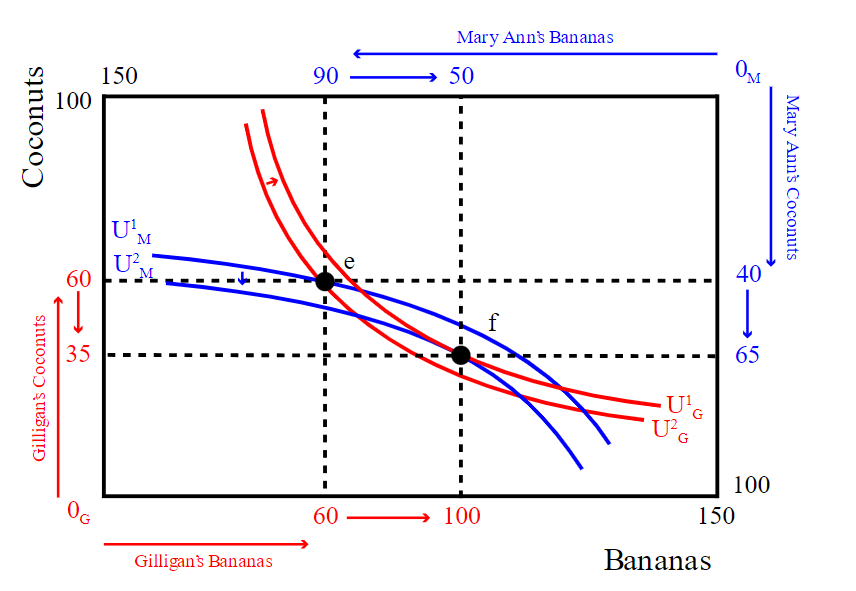
In equilibrium, the price line is tangent to the consumers’ indifference curves at point f as well as to the PPF at point a. Thus a competitive equilibrium is reached. Consumers are maximizing their utilities at point f, producers are maximizing their returns at point a, and supply equals demand in both markets: Gilligan consumes 100 bananas and 35 coconuts; Mary Ann consumes 50 bananas and 65 coconuts; and the combined demand for both, 150 bananas and 100 coconuts, exactly equals the supply.
14.5 POLICY EXAMPLE SHOULD THE GOVERNMENT TRY TO ADDRESS GROWING INEQUALITY THROUGH TAXES AND TRANSFERS?
Learning Objective 14.5: Show how any redistribution of resources leads to a Pareto-efficient competitive equilibrium.
Income inequality is the outcome of markets and society. An unequal distribution of societal resources can be represented in the abstract through the use of Edgeworth box analysis. Though an Edgeworth box represents only two people and two goods, the insight generalizes to many people and many goods. We can represent inequality by an initial distribution of societal resources that gives most of them to only one person, as shown in figure 14.19.
Figure 14.19 A tax and transfer scheme to address initial inequality
Figure 14.19 shows an economy where there are two people, 1 and 2, and two goods, A and B. The initial allocation is at A, where person 1 has most of both goods. The competitive equilibrium that is obtained from this allocation is at B, which is still highly unequal. To address this, a tax and transfer scheme could be implemented by taking away some of the initial allocation of A and B from 1 and transferring them to 2. This is shown in figure 14.19 as the movement from allocation a to the allocation x. The government that does this is not able to know all the societal preferences and thus is unable to know where the competitive equilibriums are—they do not know the contract curve. So their tax and transfer scheme does not get them directly to a competitive equilibrium. However, the first and second welfare theorems ensure that the competitive equilibrium is Pareto efficient and that any Pareto-efficient allocation can be obtained through a redistribution of the initial endowment.
So we can see in the figure that the new allocation x will lead to the Pareto-efficient outcome y. This suggests that there is no efficiency loss from a tax and transfer scheme. Person 1 is worse off than before the taxes and transfers, and person 2 is better off. Inequality has been addressed, but whether society is better off because of it is something that would require additional analyses.
What we can say is that there are no wasted societal resources—there is no inefficiency. This assumes, however, that the tax and transfer scheme itself is costless, while we know that in reality, such a program would require a lot of bureaucratic costs. We also have not analyzed what a tax and transfer scheme would do to the incentive to produce. If the rich were not able to enjoy the full benefit of their labor because of an income tax, economic theory suggests that they might not work as hard, and society would produce less. How would this reveal itself? In this case, the PPF would shrink, and so would the size of the Edgeworth box, and since we assume more is better, then the opposite must also be true—less is worse.
So both the bureaucratic costs and the loss from the disincentive to work suggest that there will be a cost to this program. The benefit is a more equal distribution of income. Thus whether it is a good idea to implement, such a program depends on the relative benefits of a more equal income distribution and the costs of the program.