Welfare economics I: Efficiency and optimal allocation

 

Pareto efficiency

This efficiency criterion was developed by Vilfredo Pareto in his book “Manual of Political Economy”, 1906. An allocation of goods is Pareto optimal when there is no possibility of redistribution in a way where at least one individual would be better off while no other individual ends up worse off.

A definition can also be made in two steps:

-a change from situation A to B is a Pareto improvement if at least one individual is better off without making other individuals worse off;

-B is Pareto optimal if there is no possible Pareto improvement.

This can be easily understood using an Edgeworth box. Starting from point C, two Pareto improvements can be made:

-from C to D: individual 1 would increase its utility, since a further indifference curve would be reached, while individual 2 will remain with the same utility;

-from C to E: individual 2 would maintain its utility while individual 2 increases theirs.

Once we are at point either D or E, no further Pareto improvements can be made. Therefore, D and E are Pareto optimal.

Following the same steps for every indifference curve, we can say that every point in which indifference curves from different individuals are tangent is Pareto optimal. The curve that links these infinite Pareto optima is called the contract curve.

Edgeworth box

In 1881, Francis Y. Edgeworth came up with a way of representing, using the same axis, indifference curves and the corresponding contract curve in his book “Mathematical Psychics: an Essay on the Application of Mathematics to the Moral Sciences”. However, the representation given, using as an example the work being done by Friday and wages being paid by Robinson Crusoe, was not the one we commonly know nowadays.

It was Vilfredo Pareto, in his book “Manual of Political Economy”, 1906, who developed Edgeworth’s ideas into a more understandable and simpler diagram, which today we call the Edgeworth box.

This diagram is widely used in welfare economics, game theory or general equilibrium theory, to name a few. It is easy to draw and can be easily explained. In the adjacent image, we can see two examples of an Edgeworth box, and how it is drawn.

The first example is mainly used for welfare economics and distribution matters. As we see, this “box” is formed using two sets of typical indifference maps, which in this case represent the indifference curves of agents A (green) and B (red), who must choose quantities of goods x and y. When the indifference map of agent B is rotated, and put on top of the map of agent A, the box is formed. When indifference curves are tangent to each other, which is the case in this example, a contract curve (blue) can be drawn using these tangency points.

Our second example is mainly used to explain Ricardian trade theory graphically. In this case, we draw the production-possibility frontier for countries 1 (green) and 2 (red). When we rotate the diagram of country 2, we end up with an Edgeworth box, which here will help understand how great the gains of international trade are and therefore helps illustrate how trade is not a sum zero game.

Video – Edgeworth box:

Production possibility frontier

The production possibility frontier (PPF) represents the quantity of output that can be obtained for a certain quantity of inputs using a given technology. Depending on the technology, the PPF will have a certain shape.

As you can see on the adjacent figure, this PPF (blue curve) slopes downwards. This slope, which equals the marginal rate of transformation between X and Y, shows us how, in order to increase the output X, the quantity of Y must decrease. In fact, the marginal rate of transformation measures the tradeoff of producing more X in terms of Y.

This frontier determines the maximum output (of both X and Y) that can be obtained given the technology. Production at point A will produce more quantity of Y and less of X than production at point B. However, both are technically efficient, since they maximize the output. For example, production at point C is technically inefficient because, at any point on the PPF, more combined output is produced using given the technology. Also, point D is unattainable given the technology, being this is the reason why it is outside the PPF.

The PPF can be derived from the contract curve on an Edgeworth box. In this box, we see the quantity of inputs (K, L) being used in the production of each good (X,Y). In fact, we can see how, for each quantity of each product, the quantity of each input can change. The isoquants (green curve for X, red for Y) determine how much a certain input has to increase in order to compensate the decrease in the other input, maintaining the quantity of output produced unaltered. The slope of these curves is given by the marginal rate of technical substitution of each output.

The points where the isoquants of different outputs combination intersect, which are Pareto-optimal, allow us to draw the contract curve, from which the PPF can be derived. Since the technology is given, only one PPF can be derived from the contract curve (as opposed to the case of the utility possibility frontier).

 

Video – Production possibility frontier:

General equilibrium

A market system is in competitive equilibrium when prices are set in such a way that the market clears, or in other words, demand and supply are equalised. At this competitive equilibrium, firms’ profits will necessarily have to be zero, because otherwise there will be new firms that, attracted by the profits, would enter the market increasing supply and pushing prices down. Following the first fundamental theorem of welfare economics, this equilibrium must be Pareto efficient. Both will have a fundamental relation as a mechanism for determining optimal production, consumption and exchange.

Initial approach:

Let’s consider an economy where there are:

Two factors of production: capital (K) and labour (L).

Two goods: good X and good Y.

Two agents: A and B

The economic problem that is faced needs to find the most adequate allocation of factors of production in order to produce goods X and Y and how these goods will be distributed amongst consumers A and B. This configuration will be such that there will be no other feasible configuration that will allow an increase in any individual’s welfare without decreasing the other individual’s welfare.

In order to achieve Pareto optimality, a certain set of assumptions need to be held.

-The production function needs to be continuous, differentiable, and strictly concave. This will result in a convex set of production possibilities, also known as production possibility frontier Its shape shows an increasing opportunity cost as we need to use a higher number of resources in order to produce a larger amount of a certain good.

-Consumers’ preferences need to be monotonic, convex and continuous, showing how individuals’ welfare increases with a greater amount of goods, but with a decreasing marginal utility.

–Perfect and free availability of information.

-There has to be an absence of externalities and public goods so the utility of individuals depends directly and uniquely from their possession of goods X and Y.

Production optimisation

The optimisation problem in production relies in the maximisation of total output production taking into consideration that it is subject to a limited amount of capital and labour. Analytically,

We can start by looking at the production of goods X and Y as two different optimisation problems. The firm will have to decide what quantity of capital and labour allocate to the production of good X, as shown on the left side of the diagram below, but also what quantity of capital and labour assign to the production of good Y, as shown on the right. These curves are the isoquants corresponding to each production process. 

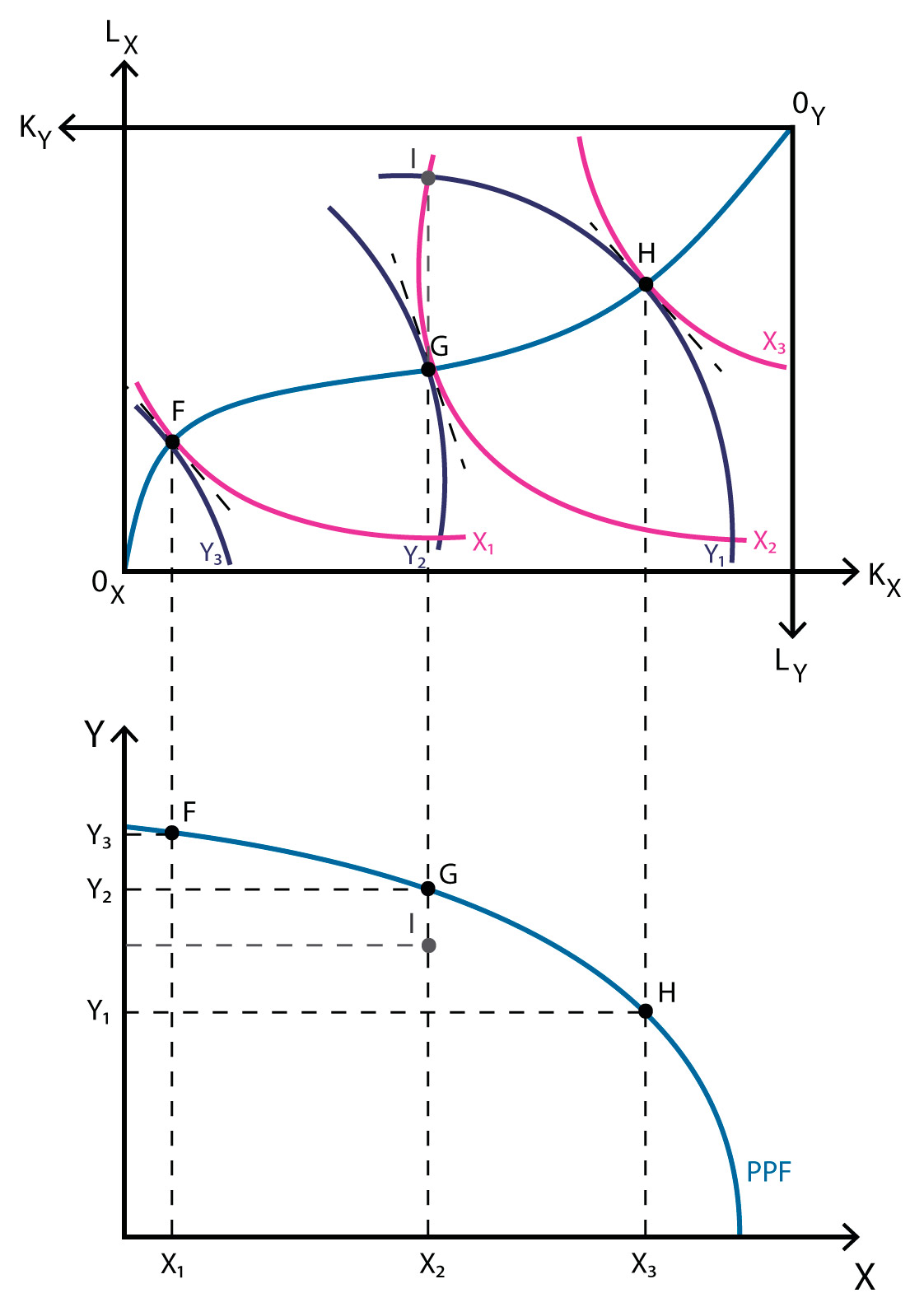
These two diagrams can be plotted together using what is known as the Edgeworth box, which makes it easier to compare quantities of capital and labour used, while also comparing quantities of goods X and Y being produced. Indeed, it’s not only easier to analyse, but also makes more sense, since the total available quantities of capital and labour are given. 

The solution to this problem is related to the marginal rate of technical substitution (MRTS). A higher efficiency will be achieved if the reallocation of a unit of labour or capital from one good to another leads to a higher production of the former. When the marginal rate of technical substitution is equal for both goods, it means that all available inputs are being used, which translates into a purely efficient production process. 

Graphically, if we plot all these points we construct what is known as the contract curve (blue curve in the Edgeworth box). These represent all Pareto efficient distributions, such as F, G or H. I is not Pareto efficient, since going from I to either G or H would result in an increase in the production of one of the goods without giving up the production of the other.  From this curve we can derive the production possibility frontier, which shows the quantities of goods X and Y being produced, as shown in the following diagram. It must be noted that both the contract curve and its derivative, the production possibility frontier, show all the solutions that are Pareto efficient from the firm’s point of view. Only when considering input and output prices will we be able to determine a unique solution (because of the concavity of the production possibility frontier).

Consumption optimisation

Bundles of goods cannot be ranked in a reliable way without knowledge of the distribution of the products, especially if a bundle has different amounts of each good. There may be some bundles that have more products of a good but less of another. The optimisation problem will be to maximise the utility of individuals A and B subject to a limited total amount of goods X and Y. Analytically,

In this case we have to achieve the optimal distribution of two, already produced goods (X and Y) between two individuals (A and B). We can follow the same step by step method used before. Here, we’ll plot indifference curves corresponding to the amounts of goods X and Y consumed by A (on the left), and the amounts of goods consumed by B (on the right).

Again, we use the Edgeworth box to graph the different distributions that can be given between two individuals, A and B, and two goods, X and Y. The further the indifference curve is from the origin, the higher the level of utility enjoyed by the consumer. 

Although all the points in the graphic are feasible, not all are efficient, given the utilities and preferences of consumers. The indifference curves join all the points that give consumers the same level of utility. By connecting all points of tangency between the indifference curves of both individuals, the contract curve is constructed and represents all Pareto efficient allocations. The tangency between indifference curves is the point where both consumers have an equal marginal rate of substitution for goods X and Y, and are therefore not willing to trade between them, as it would result in a lower utility.

Global optimum

Until now we have only considered different parts of the economy, and not the economy as a whole. The optimisation problem faced this time is similar to the previous one, although this time an additional restriction is added, since we are here considering both production and consumption: the production level also needs to be efficient. 

As this optimisation problem is based on the previous one, we have the same marginal rate of substitution equalisation, but also these two must be equal to the marginal rate of transformation, the PPF’s slope, 

These solutions are multiple, since there are various points where the condition holds. However, if we consider output prices (given by the consideration of input prices mentioned before), we are able to consider a unique solution. In the adjacent diagram, if output prices were to be PX and PY, the equilibrium would be point E. However, if output prices were instead P’X and P’Y, the equilibrium would be point E’.

Let’s say that prices are set at PX and PY, and that the equilibrium point is E, as seen in the diagram below. Consumers A and B will consume both goods X and Y in different amounts. These amounts are given by the equilibrium in consumption, point E on the contract curve. We have also equilibrium in the production process, given by point E on the production possibility frontier. We know this is a general equilibrium because the marginal rate of substitution is equal to the marginal rate of transformation; or, in other words, the slopes of the indifference curves are equal to the slopes of the production possibility frontier.

Competitive markets result in an equilibrium position such that it is not possible to make a change in the allocation without making someone else worse-off. In reality there are many Pareto optimums and we cannot state that one is better than the other. Even if one consumer got all of the production and the other one none, we cannot say it is an inefficient distribution if all resources are being used efficiently. This is the reason why some economists believe it is an incomplete criterion. However, there are others, such as Milton Friedman and the advocates of the Chicago School, for whom this proves that the economy will act efficiently without the need of government intervention.

Fundamental theorems

There are two fundamental theorems of welfare economics.

 

-First fundamental theorem of welfare economics (also known as the “Invisible Hand Theorem”):

any competitive equilibrium leads to a Pareto efficient allocation of resources.

The main idea here is that markets lead to social optimum. Thus, no intervention of the government is required, and it should adopt only “laissez faire” policies. However, those who support government intervention say that the assumptions needed in order for this theorem to work, are rarely seen in real life.

It must be noted that a situation where someone holds every good and the rest of the population holds none, is a Pareto efficient distribution. However, this situation can hardly be considered as perfect under any welfare definition. The second theorem allows a more reliable definition of welfare

 

-Second fundamental theorem of welfare economics:

any efficient allocation can be attained by a competitive equilibrium, given the market mechanisms leading to redistribution.

This theorem is important because it allows for a separation of efficiency and distribution matters. Those supporting government intervention will ask for wealth redistribution policies.

https://cutt.ly/B7XTS8D

Welfare economics I: Definition and main economists

 

Summary

Welfare economics analyses different states in which markets or the economy can be. Its main objective is to find an indicator or measure in order to guarantee that markets are behaving optimally, thus also guaranteeing that consumer welfare is as high as possible. In this Learning Path, we learn about the basics of welfare economics.

Welfare economics are a part of normative economics which objective is to evaluate different situations of a given economic system, in order to choose the best one.

Its study can be traced back to Adam Smith, who related an increase of welfare with an increase on production, and to Jeremy Bentham, whose utilitarian views made him think that welfare was equal to the sum of individuals utilities or, in other words, to a “social” utility.

Traditional welfare economics is based on the work of three neoclassical economists. Alfred Marshall stated that consumer’s welfare was the consumer’s surplus, and therefore was measurable in monetary units. Vilfredo Pareto would criticize this cardinal view, and would be the economist who built a true theory of welfare economics in his book “Manual of Political Economy”, 1906: based on the principles of unanimity and individualism, he designed what nowadays is known as the Pareto Optimality, which would become the core of welfare economics. Later, Pigou wrote “The Economics of Welfare”, 1920, stating that a definition of social welfare must include both efficiency and equity.

During the XXth century, welfare economics developed quickly. Nicholas Kaldor and John Hicks’ compensation criteria, and its following critics by Scitovsky, Little and Paul Samuelson, which aim was to find some way of classification of different optima. Also Bergson’s social welfare function, and Kenneth Arrow’s impossibility theorem, proving the former could not be identified. The theory of second best, developed by Lipsey and Lancaster, aimed at finding an optimum when Pareto optimality could not be found. Finally, the increasing use of cost-benefit analysis marks the validity of welfare economics nowadays.

Arthur C. Pigou

Pigou was a British economist (1877-1959), disciple of Alfred Marshall, whom he succeeded as a professor at Cambridge. Pigou is remembered above all as a precursor of welfare economics, for his books “Wealth and Welfare”, 1912, and “The Economics of Welfare”, 1920, in which he used measures of national income and its distribution in order to understand how wealth and welfare are related. He is also remembered for making a distinction between different degrees of price discrimination.

Being part of the Cambridge school, Pigou used common tools derived from neoclassical economics, such as marginalism, amongst others.

Vilfredo Pareto

Pareto was an economist and sociologist of Italian origin, born in Paris (1848-1923), who taught at the University of Lausanne, as well as previously did his mentor, Léon Walras. They both were part of the Lausanne School, which is considered, along with the Austrian School, as the birthplace of marginalism and neoclassical economics.

His chief works were “Course of Political Economy”, 1896-97, and “Manual of Political Economy”, 1906. Among Pareto’s contributions, we can highlight the graphical development of Edgeworth box, as well as an improvement on the way indifference curves are drawn, and studies on the personal distribution of income.

In his studies of the late nineteenth century, Pareto found some regularity in the personal distribution of income in different countries. From that regularity, he determined a series of economic and sociological conclusions, which became known afterwards as Pareto’s Laws. He also studied some regularities in businesses, where concentration was the explanation for the fact that many companies get 80% of their revenue from only 20% of its products.

Nowadays, however, he is mostly known for the Pareto optimal, a notion widely used in game theory and welfare economics.

https://cutt.ly/s4JtoZW

Economics Summary

 Economics is concerned with the optimal distribution of scarce resources within society. For example, economics is concerned with how individual decisions like how firms produce goods and which goods people buy. An important element in economics is concerned with the extent to which governments can intervene in the economy to improve economic welfare. Economics is also concerned with wider issues such as economic growth and unemployment – issues that affect the whole of society.

The most basic model in economics concerns how the price and quantity of goods and services is determined. If there was a shortage of a good – queues of people forming, then there is an incentive for firms to increase price. This increase in price reduces demand and encourages supply. Prices change until markets reach equilibrium.  Adam Smith referred to the ‘invisible hand’ of the market for explaining how prices adjust.

If demand for a good rose, we observe that this usually leads to a higher price. This higher price, in turn, encourages firms to supply more. This simple model helps explain a whole variety of different issues and topics. For example, we can use supply and demand to explain wage differentials. A lawyer can command a high wage because the number of qualified lawyers is very low. Cleaners tend to get lower wages because there are many more people with necessary qualifications.

Behaviour

Economics is concerned with decisions that agents (firms and consumers) make. For example, classical economics generally assumes that people wish to maximise their well-being; i.e. we assume firms wish to maximise profits and consumers wish to maximise their utility (happiness)

However, the real world is more complicated. Not all firms wish to maximise profits; they may seek to maximise market share or pursue other social/environmental objectives. Also, people may not be rational but get caught up in irrational booms and busts (e.g. stock market booms, housing  booms, dot com bubbles). Therefore there is a branch of economics known as behavioural economics. In recent years, this branch of economics has increased (Richard Thaler was awarded the Nobel Prize in Economics (2017) for his work on behavioural economics, which included work on

Dual-system theory – the idea we have two decision making elements. One is impulsive, the other is more rational, cognitive and analytical. Similar to ‘hot-cold’ states.

Mental accounting – how individuals separate their budget into different accounts, limiting spending on particular aspects of expenditure.

Prospect theory – the idea we suffer comparatively more from losses than gains. It also places emphasis on a relative starting point. We judge utility from our loss/gain – rather than our finishing point.

Macro Economics

Macroeconomics is a term relating to nationwide economic problems. For example, the rate of inflation in a country measures the average increase in prices. Higher inflation affects both savers and borrowers and can influence living standards. Economic growth is another key factor that can determine living standards. Higher economic growth can lead to improved living standards and lower rates of unemployment. A recession (negative economic growth) can lead to the opposite. Macroeconomics

Government Intervention in the Economy

A continual debate in economics is the extent to which governments intervene in the economy. On the one hand, free-market economists argue government intervention should be very limited (e.g. the protection of private property, national defence). The argument of free market economics is that governments tend to be inefficient, they don’t have the same incentives to produce what people want and need. If you leave it to markets, the ‘invisible hand’ automatically responds to changes in demand to provide goods that people want.

On the other hand, other economists argue that the free market actually creates many problems. In a free market, we may have monopolies, inequality, under-provision of important public services. Therefore to improve economic welfare, there is a necessity for governments to raise tax and spend on public goods not provided by the free market. Markets vs Government Intervention

Goods with positive externalities (e.g. trains which reduce pollution and congestion) may be under-consumed in a free market. A government can raise taxes and subsidise these positive externalities.

A big issue is to what extent should a government intervene in the economy?

What is the goal of economics?

Classical economic theory assumes the goal of economics is to maximise utility (satisfaction of material wants). This emerged from the philosophy of utilitarianism. It is an assumption firms seek to maximise profits and consumers seek to maximise consumption.

Rational economic man

However, in recent years, more economists have challenged whether economic welfare is the same as maximising production and consumption. For example, with a diminishing marginal utility of wealth, we may get more happiness from increasing leisure time and looking after the environment

DIminishing returns to wealth/income

Happiness economics looks at ways to increase happiness – rather than net welfare.

Economic Systems

To some extent, all major economies have converged on a similar model which may be termed a ‘mixed economy’. This is a combination of free markets (no government intervention) and state provision of goods. The old Soviet Union pursued a ‘command economy’ Communist, where the government decided what to produce, how to produce and for whom.

The opposite to a Command economy is a pure free market, where there is no government intervention. Within the two are mixed economies. The extent of government intervention in an economy varies significantly from 17% of GDP (Hong Kong) to over 50% in Scandinavian countries like Norway and Sweden.

https://bit.ly/3JBhJcE